使用Keras进行LSTM实战
安装依赖
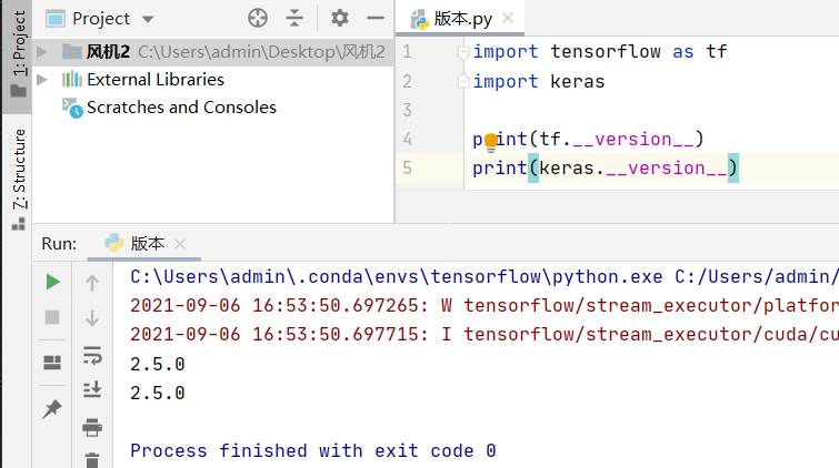
本项目采用Anaconda构建虚拟环境,配置如下:
- python 3.6(64 bit)
- tensorflow 2.5.0
- keras 2.5.0
注意版本一定不能互相冲突,详情查看:https://docs.floydhub.com/guides/environments/
实战模板
1
2
3
4
5
6
7
8
9
10
11
12
13
14
15
16
17
18
19
20
21
22
23
24
25
26
27
28
29
30
31
32
33
34
35
36
37
38
39
40
41
42
43
44
45
46
47
48
49
50
51
52
53
54
55
56
57
58
59
60
61
62
63
64
65
66
67
68
69
70
71
72
73
74
75
76
77
78
79
80
81
82
83
84
85
86
87
88
89
90
91
92
93
94
95
96
97
98
99
100
101
102
103
104
105
106
107
108
109
110
111
112
113
114
115
116
117
118
from math import sqrt
from numpy import concatenate
from pandas import read_csv
from pandas import DataFrame
from pandas import concat
from matplotlib import pyplot
from sklearn.preprocessing import MinMaxScaler
from sklearn.metrics import mean_squared_error
from keras.models import Sequential,load_model
from keras.layers import Dense
from keras.layers import LSTM
filename='data.csv'
# convert series to supervised learning
def series_to_supervised(data, n_in=1, n_out=1, dropnan=True):
n_vars = 1 if type(data) is list else data.shape[1]
df = DataFrame(data) ####Define a table.
cols, names = list(), list() #### Define two List.
for i in range(n_in, 0, -1): ####This is a loop which is carried out from n_in to 0.
cols.append(df.shift(i)) ##### Carry out a translation on df, and append members of to cols.
names += [('var%d(t-%d)' % (j + 1, i)) for j in range(n_vars)]
# forecast sequence (t, t+1, ... t+n)
for i in range(0, n_out): #### T
cols.append(df.shift(-i))
if i == 0:
names += [('var%d(t)' % (j + 1)) for j in range(n_vars)]
else:
names += [('var%d(t+%d)' % (j + 1, i)) for j in range(n_vars)]
# put it all together
agg = concat(cols, axis=1)
agg.columns = names
# drop rows with NaN values
if dropnan:
agg.dropna(inplace=True) ###delete all NULL records.
return agg
# load dataset
dataset = read_csv(filename, header=0, index_col=0)
values = dataset.values
# ensure all data is float
values = values.astype('float32')
# normalize features
scaler = MinMaxScaler(feature_range=(0, 1))
scaled = scaler.fit_transform(values)
# frame as supervised learning
reframed = series_to_supervised(scaled, 1, 1)
# 定义参数
n_hours = 1
n_features = 50
SeperatePoint=504
TheIntervalOfSample=10
TheDimensionOfInputVector=50
TheDimensionOfOutputVector=1
ThePositionOfActivePower=23
# split into train and test sets
values = reframed.values
n_train_hours = SeperatePoint * 24 * (60//TheIntervalOfSample)
train = values[:n_train_hours, :]
test = values[n_train_hours:, :]
n_obs = n_hours * n_features
# split into input and outputs
train_X, train_y = train[:, :n_obs], train[:,-1*(TheDimensionOfInputVector-ThePositionOfActivePower)]
test_X, test_y = test[:, :n_obs], test[:, -1*(TheDimensionOfInputVector-ThePositionOfActivePower)]
# reshape input to be 3D [samples, timesteps, features]
train_X = train_X.reshape((train_X.shape[0], n_hours, n_features))
test_X = test_X.reshape((test_X.shape[0], n_hours, n_features))
# design network
model = Sequential()
model.add(LSTM(TheDimensionOfInputVector, input_shape=(train_X.shape[1], train_X.shape[2]),return_sequences=True))
model.add(LSTM(TheDimensionOfInputVector,return_sequences=False))
model.add(Dense(TheDimensionOfOutputVector,activation='tanh'))
model.compile(loss='mae', optimizer='adam', metrics=['mse'])
# fit network
history = model.fit(train_X, train_y, epochs=271, batch_size=train_X.shape[0], validation_data=(test_X, test_y), verbose=1, shuffle=False)
# plot history
pyplot.plot(history.history['loss'], label='train')
pyplot.plot(history.history['val_loss'], label='test')
pyplot.legend()
# make a prediction
yhat = model.predict(test_X,verbose=1)
test_X = test_X.reshape((test_X.shape[0], n_hours*n_features))
# invert scaling for forecast
inv_yhat = concatenate((test_X[:, :ThePositionOfActivePower], yhat), axis=1)
inv_yhat = concatenate((inv_yhat, test_X[:, -1*(TheDimensionOfInputVector-ThePositionOfActivePower-1):]), axis=1)
# invert scaling for actual
test_y = test_y.reshape((len(test_y), 1))
inv_y = concatenate((test_X[:, :ThePositionOfActivePower], test_y), axis=1)
inv_y = concatenate((inv_y, test_X[:, -1*(TheDimensionOfInputVector-ThePositionOfActivePower-1):]), axis=1)
# calculate RMSE
rmse = sqrt(mean_squared_error(inv_y, inv_yhat))
print(dataset)
print('Test RMSE: %.3f' % rmse)保存/加载模型
# 确保已经安装h5py库 model.save('Model.h5') model = load_model('Model.h5')import pickle with open(Model.pickle','wb') as f pickle.dump(model,f) with open(Model.pickle','wb') as f pickle.load(model,f)1
2
2.import joblib # value=模型名 joblib.dump(filename='LR.model',value=lr) model = joblib.load(filename="LR.model")1
2
3.